📈 Theory overview
Uncertainty Quantification
In machine learning, we build predictive models from experience, by choosing the right approach for the right problem, and from the accessible data, via algorithms. Despite our best efforts, we can encounter some underlying uncertainty that could stem from various sources or causes.
- Typically, uncertainty in the machine learning process can be categorized into two types:
Aleatoric uncertainty, also known as statistical uncertainty, which is irreducible as due to the intrinsic randomness of the phenomenon being modeled
Epistemic uncertainty, also known as systematic uncertainty, which is reducible through additional information, e.g. via more data or better models
Depending on the application fields of machine learning models, uncertainty can have major impacts on performance and/or safety.
Conformal Prediction
Conformal Prediction (CP) is a set of methods to estimate uncertainty by constructing by constructing valid prediction sets, i.e. prediction sets with a probabilistic guarantee of marginal coverage. The following three features make CP methods particularly attractive: - Distribution-free. CP methods can be applied regardless of the underlying data-generating distribution. - Model-agnostic. CP works with any ML model, even with black-box models where we only have access to the outputs of the model. - Non-asymptotic. CP methods provide finite-sample probabilistic guarantees, that is, the guarantees hold without the need to assume that the number of available data grows to infinity.
Given an error rate (or significance level) \(\alpha \in (0,1)\), set by the user, a set of exchangeable (or more simply i.i.d.) train data \(\{ (X_i, Y_i) \}_{i=1}^{n}\) and a test point \((X_{new}, Y_{new})\), all of which are generated from the same joint distribution \(\mathbb{P}_{XY}\), a conformal prediction procedure uses the training data to build prediction sets \(\widehat{C}_{\alpha}(\cdot)\) so that:
Over many calibration and test sets, \(\widehat{C}_{\alpha}(X_{new})\) will contain the observed values of \(Y_{new}\) with frequency of at least \((1-\alpha)\).
Usually, the conformal prediction method uses a point-predictor model \(\widehat{f}\) and turns it into the set predictor \(C_\alpha\) via a calibration procedure. Within the conformal prediction framework, the inequality above holds for any model, any data distribution \(\mathbb{P}_{XY}\) and any training set sample size, under the following minimal assumptions: - Exchangeability. The data \((X_1,Y_i),\dots, (X_n, Y_n), (X_{new}, Y_{new})\) form an exchangeable sequence (this is a milder assumption than the data being i.i.d.). - Independence of train and calibration data. The data for the model training is independent from the data for the model calibration.
It is noteworthy that the coverage probability is marginalized over \(X\). Therefore, the CP algorithm is likely to achieve the coverage rate of \(1-\alpha\) by under-covering conditionally to some specific regions in the space of \(X\) and over-covering in other regions.
Conformal prediction can act as a post-processing procedure to attain rigorous probability coverages, as it can “conformalize” any existing predictor during or after training (black box predictors), yielding marginally valid prediction sets.
In this page, we present the most common conformal prediction methods of the literature used on regression and classification models. We also refer to Angelopoulos and Bates [2] for a hands-on introduction to conformal prediction and awesome conformal prediction github for additional ressources.
In the following, let \(D = {(X_i, Y_i)}_{i=1}^n \sim P_{XY}\) be the training data and \(\alpha \in (0, 1)\) the significance level (target maximum error rate).
Conformal Regression
Split (inductive) Conformal
The split (also called inductive) conformal prediction [8] [6] requires a hold-out calibration dataset: the dataset \(D\) is split into a proper training set \(D_{train}=\big\lbrace(X_i,Y_i), i=1,\dots,n_{train}\big\rbrace\) and an independent calibration dataset \(D_{calib}=\big\lbrace(X_i,Y_i),i=1,\dots,n_{calib}\big\rbrace\). The purpose of the calibration dataset is to estimate prediction errors and use them to build the prediction interval for a new sample \(X_{new}\).
Given a prediction model \(\widehat{f}\) trained on \(D_{train}\), the algorithm is summarized in the following:
Choose a nonconformity score \(s\), and define the error \(R\) over a sample \((X,Y)\) as \(R = s(\widehat{f}(X),Y)\). For example, one can pick the absolute deviation \(R = |\widehat{f}(X)-Y|\).
Compute the nonconformity scores on the calibration dataset: \(\mathcal{R} = \{R_i\}_{}\), where \(R_i=s(\widehat{f}(X_i), Y_i)\) for \(i=1,\dots,n_{calib}\).
Compute the error margin \(\delta_{\alpha}\) as the \((1-\alpha)(1 + 1/n_{calib})\)-th empirical quantile of \(\mathcal{R}\).
Build the prediction interval as
Note that this procedure yields a constant-width prediction interval centered on the point estimate \(\widehat{f}(X_{new})\).
In the literature, the split conformal procedure has been combined with different nonconformity scores, which produced several methods. Some of them are presented hereafter.
Locally Adaptive Conformal Regression
The locally adaptive conformal regression [7] relies on scaled nonconformity scores:
where \(\widehat{\sigma}(X_i)\) is a measure of dispersion of the nonconformity scores at \(X_i\). Usually, \(\widehat{\sigma}\) is trained to estimate the absolute prediction error \(|\widehat{f}(X)-Y|\) given \(X=x\). The prediction interval is again centered on \(\widehat{f}(X_{new})\) but the margins are scaled w.r.t the estimated local variability at \(Y | X = X_{new}\):
The prediction intervals are therefore of variable width, which is more adaptive to heteroskedascity and usually improve the conditional coverage. The price is the higher computational cost due to fitting two functions \(\widehat{f}\) and \(\widehat{\sigma}\), on the proper training set.
Leverage-Weighted Conformal Regression
The leverage-weighted conformal regression relies on the geometry of the covariates instead of learning an additional dispersion model [5]. After splitting the data into a proper training set and a calibration set, the features are standardized using the training-set statistics and the same transformation is applied to the calibration and test points. The leverage score of a sample \(x\) is defined as the squared sample Mahalanobis distance from the training centroid, scaled by :\(1/|D_{train}|\):
where \(X\) denotes the standardized training covariates. Equivalently, if \(X=U\Sigma V^\top\) is the thin singular value decomposition of \(X\), then:
Given a user-defined weighting function \(w\), the calibration nonconformity scores are:
The empirical quantile \(\delta_{\alpha}\) of these scores is then used to construct the prediction interval:
As with locally adaptive conformal regression, this yields variable-width prediction intervals. Here, the adaptation comes from the covariate geometry: calibration residuals are reweighted according to leverage, and the interval width at inference is adjusted through the same leverage-based factor.
In practice, leverage scores are sensitive to feature scales, so consistent standardization is important. The method also requires the number of training samples to exceed the number of features so that \((X^\top X)^{-1}\) is well defined.
Conformalized Quantile Regression (CQR)
Split conformal prediction can be extended to quantile predictors \(q(\cdot)\). Given a nominal error rate \(\alpha,\) and positive error rates \(\alpha_{lo}\) and \(\alpha_{hi}\) such that \(\alpha_{lo}+\alpha_{hi}=1,\) we denote by \(\widehat{q}_{\alpha_{lo}}\) and \(\widehat{q}_{1-\alpha_{hi}}\) the predictors of the \(\alpha_{lo}\) -th and \((1-\alpha_{hi})\) -th quantiles of \(Y | X.\) The quantile predictors are trained on \(D_{train}\) and calibrated on \(D_{calib}\) by using the following nonconformity score:
For example, if we set \(\alpha = 0.1\), we would fit two predictors \(\widehat{q}_{0.05}(\cdot)\) and \(\widehat{q}_{0.95}(\cdot)\) on training data \(D_{train}\) and compute the scores on \(D_{calibration}\).
Note
It is common to split evenly \(\alpha\) as: \(\alpha_{lo} = \alpha_{hi}= \frac{\alpha}{2}\), but users are free to do otherwise.
The procedure, named Conformalized Quantile Regression [9], yields the following prediction interval:
When data are exchangeable, the correction margin \(\delta_{\alpha}\) guarantees finite-sample marginal coverage for the quantile predictions, and this holds also for misspecified (i.e. “bad”) predictors.
If the fitted \(\widehat{q}_{\alpha_{lo}}\) and \(\widehat{q}_{1-\alpha_{hi}}\) approximate (empirically) well the conditional distribution \(Y | X\) of the data, we will get a small margin \(\delta_{\alpha}\): this means that on average, the prediction errors on the \(D_{calib}\) were small.
Also, if the base predictors have strong theoretical properties, our CP procedure inherits these properties of \(\widehat{q}_{}(\cdot)\). We could have an asymptotically, conditionally accurate predictor and also have a theoretically valid, distribution-free guarantee on the marginal coverage!
Cross-validation+ (CV+), Jackknife+
The leave-one-out (LOO) and the k-fold cross-validation are well known schemes used to estimate regression residuals on out-of-sample data. As shown below, one first splits the data into K partitions and then holds out a partition at a time to compute errors (nonconformity scores, in our case). Following this principle, [3] introduced the LOO jackknife+ (JP) and the k-fold Cross-validation+ (CV+). With these methods, one does not need a dedicated calibration set.
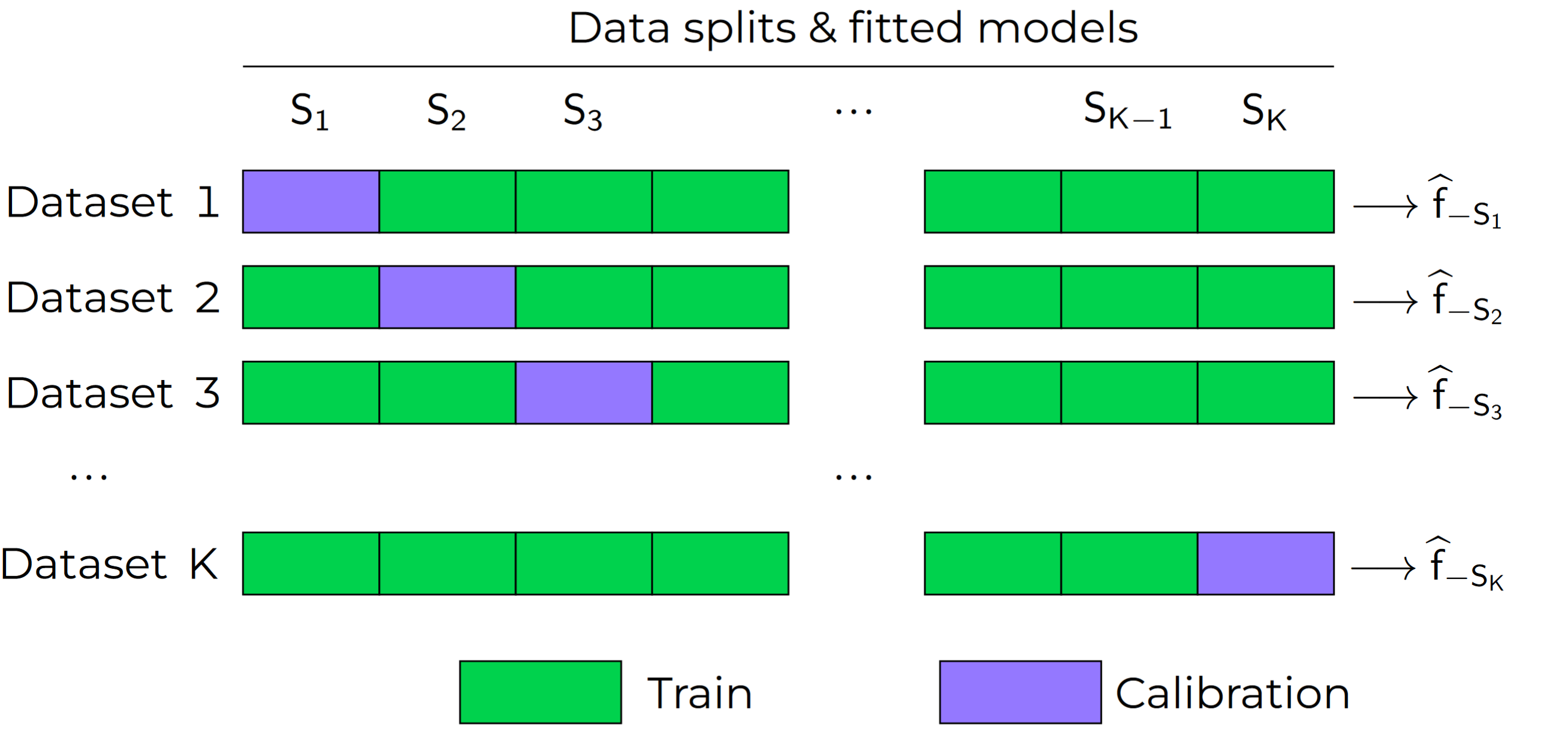
The CV+ algorithm goes as follows. Let \(n = |D_{train}|\), and let \(D_{train}\) be partitioned disjointly into the sets \(S_1, S_2, \dots, S_K\). Each training point \((X_i,Y_i) \in D_{train}\) belongs to one partition, noted as \(S_{k(i)}\).
At training, we fit and store in memory \(K\) models, referred to as \(\widehat{f}_{-S_{K}}\) to indicate that it was fitted using all data points except those in partition \(S_{K}\). Then, the conformalization step boils down to computing, for each \((X_i,Y_i) \in D_{train}\), the score:
If \(K = n\), we obtain the Jackknife+, leave-one-out version of the algorithm.
Inference
The lower and upper bounds of the prediction interval are given by:
Compute \(\bar{R}_{L} = \{ \widehat{f}_{-S_{k(i)}}(X_{new}) - R_i^{CV} \}_{i=1}^{n}\)
\(\widehat{L}_{\alpha}(X_{new}) = \lfloor \alpha (n+1) \rfloor\)-th smallest value in \(\bar{R}_{L}\) (lower bound)
Compute \(\bar{R}_{U} = \{ \widehat{f}_{-S_{k(i)}}(X_{new}) + R_i^{CV} \}_{i=1}^{n}\)
\(\widehat{U}_{\alpha}(X_{new}) = \lceil (1-\alpha) (n+1) \rceil\)-th smallest value in \(\bar{R}_{U}\) (upper bound)
Ensemble Batch Prediction Intervals (EnbPI)
Introduced in [13], the EnbPI algorithm builds prediction intervals for time series data of the form \(Y_t = f(X_t) + \epsilon_t\), where \(\epsilon_t\) are identically distributed, but not necessarily independent. Given a training dataset \(D=\lbrace (X_i, Y_i) \rbrace_{i=1}^n\) and a test set \(D_{test} = \lbrace (X_t,Y_t) \rbrace_{t=n+1}^{n_{test}}\), the EnbPI algorithm aims at constructing prediction sets for each test point \(X_t\). As with the CV+ or Jackknife+ methods, the EnbPI algorithm does not require a held-out calibration set, as it uses a bootstrap algorithm instead. Let \(\mathcal{A}\) be a training algorithm (i.e. an algorithm that maps a dataset to a predictor), and \(\phi\) an aggregation function that aggregates different individual models together, e.g. via a simple average, a bagging or an ensembling method. The algorithm EnbPI is performed in three stages:
- Training
Sample \(B\) bootstrap datasets \(S_b\), for \(b=1,\dots, B\) with replacement from \(D\).
Train \(B\) bootstrap models \(\widehat{f}^b = \mathcal{A}(S_b)\).
- Calibration
Compute the predictions on each training sample \(X_i\in D\). Only the models \(\widehat{f}^b\) where \(X_i\not\in S_b\) are used in the aggregation: \(\widehat{f}_{-i}(X_i):=\phi\big( \lbrace \widehat{f}^b(X_i) | X_i\not\in S_b\rbrace\big)\).
Compute the errors \(R_i=|Y_i-\widehat{f}_{-i}(X_i)|\), and store them as \(\mathcal{R}_1:=\lbrace R_i,i=1,\dots, n\rbrace\).
- Inference
Compute the predictions on each test sample \(X_t\in D_{test}\) by setting \(\widehat{f}_{-t}(X_t):= \frac{1}{T}\sum_{i=1}^T \widehat{f}_{-i}(X_t)\).
Update the error set: \(\mathcal R_t\) (see below).
Compute the width of the prediction intervals \(\delta_{\alpha, t}\) as the \((1-\alpha)\)-th empirical quantile of \(\mathcal{R}_t\).
The prediction interval for \(X_t\) is then given by
In order to update the error set \(\mathcal{R}_t\), a memory parameter \(s\) is employed. Every \(s\) test examples, the first \(s\) errors in the set \(\mathcal{R}\) are dropped and the errors over the last \(s\) test examples are added to the error set \(\mathcal{R}\). I.e. if \(t-n = 0\ mod\ s\) then \(\mathcal{R}_t = \lbrace R_i, i=t-n,\dots,t-1\rbrace\) and if \(t-n \neq 0\ mod\ s\) then \(\mathcal{R}_t=\mathcal{R}_{t-1}\).
Note
The EnbPI algorithm does not provide an exact probabilistic guarantee as the previous CP methods do. The guarantee provided by the EnbPI algorithm is only approximate, and holds under additional assumptions on the error process \(\epsilon_t\). However, it does not require the data to be exchangeable.
Conformal Classification
Least Ambiguous Set-Valued Classifiers (LAC)
As for the Split Conformal Regression algorithm, the LAC algorithm introduced in [11] requires us to split the dataset \(D\) into a proper training set \(D_{train}\) and an independent calibration set \(D_{calib}\). A classifier \(\widehat{\pi}\) is trained using the proper training set \(D_{train}\) only. We assume that the output of the classifier is given by the softmax scores for the different classes. I.e. for each input \(x\), the output \(\widehat{\pi}(x)=(\widehat{\pi}_1(x),\dots,\widehat{\pi}_K(x))\) is a probability vector and \(k=1,\dots, K\) represent the possible different classes in the classification task.
In order to construct the prediction sets \(\widehat{C}_\alpha\), the LAC algorithm works in two stages:
- Calibration
For each example \(X_i\) in the calibration dataset, compute the error \(R_i=1-\widehat{\pi}_{Y_i}(X_i)\), i.e. 1 minus the sofmax output of the ground truth class.
store all errors in a vector \(\mathcal{R}\).
- Inference
Compute the probability threshold \(\delta_{\alpha}\) as the \((1-\alpha)(1 + 1/n_{calib})\)-th empirical quantile of \(\mathcal{R}\).
The prediction set for a test point \(X_{new}\) is defined as
\[\widehat{C}_{\alpha}(X_{new})=\big\lbrace k \, | \, \widehat{\pi}_{k}(X_{new})\geq 1 - \delta_\alpha \big\rbrace\,.\]
Adaptive Prediction Sets (APS)
The LAC algorithm produces prediction sets that have small average size, and is known to be Bayes optimal. However, it tends to undercover in regions where the classifier is uncertain, and overcover in regions where the classifier is confident. The APS algorithm introduced in [10] aims to produce prediction sets that are more stable and have a better coverage rate. We represent by \(\widehat{\pi}_{(1)}(x)\geq \cdots\geq \widehat{\pi}_{(K)}(x)\) the softmax vector \(\widehat{\pi}\) arranged in decreasing order, i.e. \((k)\) is the index of the class having the \(k\)-th largest probability mass.
In order to construct the prediction sets \(\widehat{C}_\alpha\), the APS algorithm works in two stages:
- Calibration
For each example \(X_i\) in the calibration dataset, we compute the error \(R_i\) as the probability mass needed for reaching the true label \(Y_i\), i.e. \(R_i=\widehat{\pi}_{(1)}+\cdots+\widehat{\pi}_{(k)}\), wehere \((k)=Y_i\).
Store all errors in a vector \(\mathcal{R}\).
- Inference
Compute the probability threshold \(\delta_{\alpha}\) as the \((1-\alpha)(1 + 1/n_{calib})\)-th empirical quantile of \(\mathcal{R}\).
The prediction set for a test point \(X_{new}\) is defined as
\[\widehat{C}_{\alpha}(X_{new})=\big\lbrace (1),\dots,(k) \big\rbrace\quad \text{where}\quad k = \min\big\lbrace i : \widehat{\pi}_{(1)}+\cdots+\widehat{\pi}_{(i)}\geq \delta_\alpha\big\rbrace.\]
Regularized Adaptive Prediction Sets (RAPS)
The RAPS algorithm introduced in [1] is a modification of the APS algorithm that uses a regularization term in order to produce smaller and more stable prediction sets. Employing the same notations as for the APS algorithm above, the RAPS algorithm works in two stages:
- Calibration
For each example \(X_i\) in the calibration dataset, we compute the error \(R_i\) as the probability mass needed for reaching the true label \(Y_i\), i.e.
\[R_i=\widehat{\pi}_{(1)}+\cdots+\widehat{\pi}_{(k)} + \lambda(k-k_{reg}+1),\]where \((k)=Y_i\). The regularization term \(\lambda(k-k_{reg}+1)\) is added to the APS error, where \(\lambda\) and \(k_{reg}\) are hyperparameters.
Store all errors in a vector \(\mathcal{R}\).
- Inference
Compute the probability threshold \(\delta_{\alpha}\) as the \((1-\alpha)(1 + 1/n_{calib})\)-th empirical quantile of \(\mathcal{R}\).
The prediction set for a test point \(X_{new}\) is defined as \(\widehat{C}_{\alpha}(X_{new})=\big\lbrace (1),\dots,(k)\big\rbrace\), where
\[k = \max\big\lbrace i : \widehat{\pi}_{(1)}+\cdots+\widehat{\pi}_{(i)} + \lambda(i-k_{reg}+1) < \delta_\alpha\big\rbrace + 1.\]
Classwise Conformal Prediction
Standard conformal methods like LAC provide marginal coverage guarantees:
This means that, on average across all classes, the true label is contained in the prediction set with probability at least \(1-\alpha\). However, this marginal guarantee does not ensure that each class is covered equally well. Some classes might be over-covered while others are under-covered.
Classwise conformal prediction aims to achieve class-conditional coverage:
This is achieved by computing separate quantiles for each class during calibration, rather than a single global quantile.
The classwise LAC algorithm works as follows:
- Calibration
For each example \(X_i\) in the calibration dataset with true label \(Y_i = k\), compute the LAC score \(R_i = 1 - \widehat{\pi}_{Y_i}(X_i)\) and assign it to class \(k\).
For each class \(k\), store all scores from samples belonging to that class in \(\mathcal{R}_k\).
- Inference
For each class \(k\), compute the class-specific threshold \(\delta_{\alpha,k}\) as the \((1-\alpha)(1 + 1/n_k)\)-th empirical quantile of \(\mathcal{R}_k\), where \(n_k\) is the number of calibration samples in class \(k\).
The prediction set for a test point \(X_{new}\) is defined as
\[\widehat{C}_{\alpha}(X_{new})=\big\lbrace k \, | \, \widehat{\pi}_{k}(X_{new})\geq 1 - \delta_{\alpha,k} \big\rbrace\,.\]
For more details on classwise conformal prediction, see [12].
Conformal Anomaly Detection
Conformal prediction can be extended to handle anomaly detection, allowing us to identify data points that do not conform to the “normal” (or nominal) distribution of a dataset (see section 4.4 of [2]). The goal is to assign a statistical guarantee to the anomaly detector, ensuring that it controls the false positive rate.
To detect anomalies, we start with a model that assigns an anomaly score \(s(X)\) to each data point. Higher scores indicate a higher likelihood of being an outlier.
Assume we have a calibration dataset \(D_{calib} = \{X_i\}_{i=1}^{n_{calib}}\) consisting of nominal (non-anomalous) examples. The conformal anomaly detection algorithm proceeds as follows:
- Calibration
For each example \(X_i\) in the calibration dataset, we compute the nonconformity score as the anomaly score provided by the model, i.e. \(R_i = s(X_i)\).
Store all nonconformity scores in a vector \(\mathcal{R}\).
Inference
Compute the anomaly score threshold \(\delta_{\alpha}\) as the \((1-\alpha)(1 + 1/n_{calib})\)-th empirical quantile of \(\mathcal{R}\).
For a new test point \(X_{new}\), the conformalized anomaly detector classifies it as:
\[\begin{split}\widehat{C}_{\alpha} = \begin{cases} \text{Normal} & \text{if } s(X_{new}) \leq \delta_{\alpha} \\ \text{Anomaly} & \text{if } s(X_{new}) > \delta_{\alpha} \end{cases}\end{split}\]
Conformal anomaly detection provides an error control guarantee, meaning that under the assumption of exchangeability, the probability of a false positive (labeling a norminal instance as an anomaly) is bounded by \(\alpha\).
Conformal Object Detection
Conformal prediction can be extended to object detection tasks, where the goal is to predict the bounding boxes of objects in an image with a probabilistic guarantee [4]. There are many way to formulate Conformal Object Detection, in PUNCC we have implemented the so-called Split-Boxwise Conformal Object Detection algorithm. Here, we conformalize predicted bounding boxes by adjusting their coordinates with a margin that depends on the nonconformity scores of the calibration dataset. A bounding box is charecterized by its lower-left corner and upper-right corner coordinates, i.e. \(Y = (Y^{x_\min}, Y^{y_\min}, Y^{x_\max}, Y^{y_\max})\). The algorithm computes the nonconformity scores for each coordinate separately, and computes the prediction interval for each coordinate independently. By using a Bonferroni-type correction, the algorithm ensures that on average \(1-\alpha\) of the predicted bounding boxes contain the true bounding box. The algorithm is summarized as follows:
Calibration
For each predicted box \(\widehat{Y}_i\) in the calibration dataset, we compute the nonconformity score separately for each of the four coordinates, tha is, \(R_i^j = \widehat{Y}_i^j - Y_i^j\) for \(j\in\lbrace x_\min, y_\min, x_\max, y_\max\rbrace\).
Store all nonconformity scores in vectors \(\mathcal{R^j}\) for \(j\in\lbrace x_\min, y_\min, x_\max, y_\max\rbrace\).
Inference
Compute the nonconformity scores thresholds \(\delta_{\alpha/4}^j\) as the \((1-\frac{\alpha}{4})(1 + 1/n_{calib})\)-th empirical quantile of \(\mathcal{R^j}\) for \(j\in\lbrace x_\min, y_\min, x_\max, y_\max\rbrace\).
For a new test predicted box \(\widehat{Y}_{new}\), the conformalized object detector predicts the adjusted bounding box with coordinates:
\[\widehat{C}_{\alpha} = \big\lbrace \text{box with coordinates} \, \widehat{Y}_{new}^j - \delta_{\alpha/4}^j \, \text{for} \, j\in\lbrace x_\min, y_\min, x_\max, y_\max\rbrace \big\rbrace.\]
In order to perform the calibration step, we need to pass to the algorithm a series of predicted bounding boxes and their corresponding ground truth bounding boxes. In order to provide the calibration algorithm with a list of pairs of predicted and ground truth bounding boxes, we can use a matching algorithm like the Hungarian matching algorithm that will maximize the intersection over union (IoU) between the predicted and ground truth bounding boxes.
References
Anastasios Angelopoulos, Stephen Bates, Jitendra Malik, and Michael I Jordan. Uncertainty sets for image classifiers using conformal prediction. arXiv preprint arXiv:2009.14193, 2020.
Anastasios N Angelopoulos, Stephen Bates, and others. Conformal prediction: a gentle introduction. Foundations and trends® in machine learning, 16(4):494–591, 2023.
Rina Foygel Barber, Emmanuel J Candes, Aaditya Ramdas, and Ryan J Tibshirani. Predictive inference with the jackknife+. The Annals of Statistics, 49(1):486–507, 2021.
Florence De Grancey, Jean-Luc Adam, Lucian Alecu, Sébastien Gerchinovitz, Franck Mamalet, and David Vigouroux. Object detection with probabilistic guarantees: a conformal prediction approach. In International Conference on Computer Safety, Reliability, and Security, 316–329. Springer, 2022.
Shreyas Fadnavis. Leverage-weighted conformal prediction. arXiv preprint arXiv:2602.12693, 2026.
Jing Lei, Max G'Sell, Alessandro Rinaldo, Ryan J Tibshirani, and Larry Wasserman. Distribution-free predictive inference for regression. Journal of the American Statistical Association, 113(523):1094–1111, 2018.
Harris Papadopoulos, Alex Gammerman, and Volodya Vovk. Normalized nonconformity measures for regression conformal prediction. In Proceedings of the IASTED International Conference on Artificial Intelligence and Applications (AIA 2008), 64–69. 2008.
Harris Papadopoulos, Kostas Proedrou, Volodya Vovk, and Alex Gammerman. Inductive confidence machines for regression. In European conference on machine learning, 345–356. Springer, 2002.
Yaniv Romano, Evan Patterson, and Emmanuel Candes. Conformalized quantile regression. Advances in neural information processing systems, 2019.
Yaniv Romano, Matteo Sesia, and Emmanuel Candes. Classification with valid and adaptive coverage. Advances in neural information processing systems, 33:3581–3591, 2020.
Mauricio Sadinle, Jing Lei, and Larry Wasserman. Least ambiguous set-valued classifiers with bounded error levels. Journal of the American Statistical Association, 114(525):223–234, 2019.
Vladimir Vovk. Conditional validity of inductive conformal predictors. In Proceedings of the Asian Conference on Machine Learning, 475–490. PMLR, 2012.
Chen Xu and Yao Xie. Conformal prediction interval for dynamic time-series. In International Conference on Machine Learning, 11559–11569. PMLR, 2021.