🚀 Quickstart

📈 Conformal Regression

Let’s consider a simple regression problem on diabetes data provided in Scikit-learn. We want to evaluate the uncertainty associated with the prediction using inductive (or split) conformal prediction.

💾 Diabetes Dataset

The dataset contains information about 442 diabetes patients. The goal is predict from physiological variables a quantitative measure of disease progression in one year.

• There are ten standardized features corresponding to the age, sex, body mass index, average blood pressure, and six blood serum measurements.

• The target is the measure of diabetes progression during one year for each patient.

for more information, check the official documentation.

from sklearn import datasets

# Load the diabetes dataset
diabetes_X, diabetes_y = datasets.load_diabetes(return_X_y=True)

print(f"Features shape: {diabetes_X.shape}")
print(f"Target's shape: {diabetes_y.shape}")

Features shape: (442, 10)
Target's shape: (442,)

From all the features, we want our model to capture only the link between body mass index and the evolution of the disease.

import numpy as np

# Use only BMI feature
diabetes_X = diabetes_X[:, 2, np.newaxis]

By construction, data are indepent and identically distributed (i.i.d).

Great, we fullfill the prerequisites to apply conformal prediction 👏!

The next step is spliting the data into three subsets:

• Fit subset \({\cal D_{fit}}\) to train the model.

• Calibration subset \({\cal D_{calib}}\) on which nonconformity scores are computed.

• Test subset \({\cal D_{test}}\) on which the prediction intervals are estimated.

Warning

Rigorously, for the probabilistic guarantee to hold, the calibration subset needs to be sampled for each new example in the test set.

The following code implements all the aforementioned steps:

# Split the data into training/testing sets
X_train = diabetes_X[:-100]
X_test = diabetes_X[-100:]

# Split the targets into training/testing sets
y_train = diabetes_y[:-100]
y_test = diabetes_y[-100:]

# Split fit and calibration data
X_fit, X_calib = X_train[:-100], X_train[-100:]
y_fit, y_calib = y_train[:-100], y_train[-100:]

🔮 Prediction model

We consider a simple linear regression model from scikit-learn regression module, to be trained later on \({\cal D_{fit}}\):

from sklearn import linear_model

# Create linear regression model
lin_reg_model = linear_model.LinearRegression()

Such model needs to be wrapped in a wrapper provided in the module deel.puncc.api.prediction. The wrapper makes it possible to use various models from different ML/DL libraries such as Scikit-learn, Keras or XGBoost. An example of conformal classification with keras models is provided later in this page. For more information about model wrappers and supported ML/DL libraries, checkout the documentation.

For a linear regression from scikit-learn, we use deel.puncc.api.prediction.BasePredictor as follows:

from deel.puncc.api.prediction import BasePredictor

# Create a predictor to wrap the linear regression model defined earlier
lin_reg_predictor =  BasePredictor(lin_reg_model)

⚙️ Conformal prediction

For this example, the prediction intervals are obtained throught the split conformal prediction method provided by the class deel.puncc.regression.SplitCP. Other methods are presented here.

from deel.puncc.regression import SplitCP

# Coverage target is 1-alpha = 90%
alpha=.1

# Instanciate the split cp wrapper around the linear predictor.
# The `train` argument is set to True such that the linear model is trained
# before the calibration. You can initialize it to False if the model is
# already trained and you want to save time.
split_cp = SplitCP(lin_reg_predictor, train=True)

# Train model (if argument `train` is True) on the fitting dataset and
# compute the residuals on the calibration dataset.
split_cp.fit(X_fit=X_fit, y_fit=y_fit, X_calib=X_calib, y_calib=y_calib)

# The `predict` returns the output of the linear model `y_pred` and
# the calibrated interval [`y_pred_lower`, `y_pred_upper`].
y_pred, y_pred_lower, y_pred_upper = split_cp.predict(X_test, alpha=alpha)

The library provides several metrics in deel.puncc.metrics to evaluate the conformalization procedure. Below, we compute the average empirical coverage and the average empirical width of the prediction intervals on the test examples:

from deel.puncc import metrics

coverage = metrics.regression_mean_coverage(y_test, y_pred_lower, y_pred_upper)
width = metrics.regression_sharpness(y_pred_lower=y_pred_lower,
                                     y_pred_upper=y_pred_upper)
print(f"Marginal coverage: {np.round(coverage, 2)}")
print(f"Average width: {np.round(width, 2)}")

Marginal coverage: 0.95
Average width: 211.38

In addition, puncc provides plotting tools in deel.puncc.plotting to visualize the prediction intervals and whether or not the observations are covered:

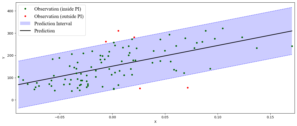
90%-prediction interval with the split conformal prediction method

📊 Conformal Classification

Let’s tackle the classic problem of MNIST handwritten digits classification. The goal is to evaluate through conformal prediction the uncertainty associated with predictive classifiers.

💾 MNIST Dataset

MNIST dataset contains a large number of \(28 \times 28\) digit images to which are associated digit labels. As the data generating process is considered i.i.d (check this post), conformal prediction is applicable 👏.

We split the data into three subsets:

• Fit subset \({\cal D_{fit}}\) to train the model.

• Calibration subset \({\cal D_{calib}}\) on which nonconformity scores are computed.

• Test subset \({\cal D_{test}}\) on which the prediction intervals are estimated.

Warning

Rigorously, for the probabilistic guarantee to hold, the calibration subset needs to be sampled for each new example in the test set.

In addition to data preprocessing, the following code implements the aforementioned steps:

from tensorflow.keras.datasets import mnist
from tensorflow.keras.utils import to_categorical

# Load MNIST Database
(X_train, y_train), (X_test, y_test) = mnist.load_data()

# Preprocessing: reshaping and standardization
X_train = X_train.reshape((len(X_train), 28, 28))
X_train = X_train.astype('float32') / 255
X_test = X_test.reshape((len(X_test), 28 , 28))
X_test = X_test.astype('float32') / 255

# Split fit and calib datasets
X_fit, X_calib  = X_train[:50000], X_train[50000:]
y_fit, y_calib  = y_train[:50000], y_train[50000:]

# One hot encoding of classes
y_fit_cat = to_categorical(y_fit)
y_calib_cat = to_categorical(y_calib)
y_test_cat = to_categorical(y_test)

🔮 Prediction Model

We consider a convnet defined as follows:

from tensorflow import random
from tensorflow import keras
from tensorflow.keras import layers

random.set_seed(42)

# Classification model: convnet composed of two convolution/pooling layers
# and a dense output layer
nn_model = keras.Sequential(
   [
      keras.Input(shape=(28, 28, 1)),
      layers.Conv2D(16, kernel_size=(3, 3), activation="relu"),
      layers.MaxPooling2D(pool_size=(2, 2)),
      layers.Conv2D(32, kernel_size=(3, 3), activation="relu"),
      layers.MaxPooling2D(pool_size=(2, 2)),
      layers.Flatten(),
      layers.Dense(10, activation="softmax"),
   ]
)

For the convnet above, we use deel.puncc.api.prediction.BasePredictor as wrapper. Note that our model is not already trained (is_trained = False), we need to provide the compilation config to the constructor:

from deel.puncc.api.prediction import BasePredictor

# The compilation details are gathered in a dictionnary
compile_kwargs = {"optimizer":"adam", "loss":"categorical_crossentropy","metrics":["accuracy"]}

# Create a predictor to wrap the convnet model defined earlier
class_predictor = BasePredictor(nn_model, is_trained=False, **compile_kwargs)

⚙️ Conformal prediction

The RAPS procedure is chosen to conformalize our convnet classifier. Such algorithm has two hyparameters \(\lambda\) and \(k_{reg}\) that encourage smaller prediction sets.

To start off gently, we will ignore the regularization term (\(\lambda = 0\)), which simply turns the procedure into APS:

from deel.puncc.classification import RAPS

# Coverage target is 1-alpha = 90%
alpha = .1

# Instanciate the RAPS wrapper around the convnet predictor.
# The `train` argument is set to True such that the convnet model is trained
# before the calibration. You can initialize it to False if the model is
# already trained and you want to save time.
aps_cp = RAPS(class_predictor, lambd=0, train=True)

# The train details of the convnet are gathered in a dictionnary
fit_kwargs = {"epochs":2, "batch_size":256, "validation_split": .1, "verbose":1}

# Train model (argument `train` is True) on the fitting dataset (w.r.t. the fit config)
# and compute the residuals on the calibration dataset.
aps_cp.fit(X_fit=X_fit, y_fit=y_fit_cat, X_calib=X_calib, y_calib=y_calib, **fit_kwargs)

# The `predict` returns the output of the convnet model `y_pred` and
# the calibrated prediction set `set_pred`.
y_pred, set_pred = aps_cp.predict(X_test, alpha=alpha)

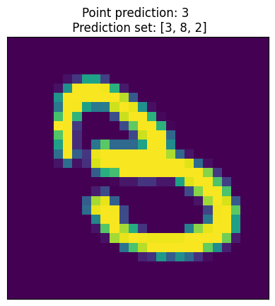
Let’s visualize an example of point prediction and set prediction.

import matplotlib.pyplot as plt

sample = 18

plt.imshow(X_test[sample].reshape((28,28)))
plt.title(f"Point prediction: {np.argmax(y_pred[sample])} \n Prediction set: {set_pred[sample]}")

The library provides several metrics in deel.puncc.metrics to evaluate the conformalization procedure. Below, we compute the average empirical coverage and the average empirical size of the prediction sets on the test examples:

from deel.puncc import metrics

mean_coverage = metrics.classification_mean_coverage(y_test, set_pred)
mean_size = metrics.classification_mean_size(set_pred)

print(f"Empirical coverage : {mean_coverage:.2f}")
print(f"Average set size : {mean_size:.2f}")

Empirical coverage : 0.90
Average set size : 1.03

🚩 Conformal Anomaly Detection

Let’s consider the two moons dataset and a collection of data points randomly scattered across a plane. Among these points, some will stand out as outliers, deviating significantly from the crescent-shaped clusters. Using an isolation forest algorithm, we generate anomaly scores for each data point. Subsequently, we wrap the model with conformal anomaly detection to calibrate the detection threshold. This ensures that the False Detection Rate (FDR) remains below the user-specified threshold \(\\alpha\).

💾 Two moons Dataset

The two moons dataset is a synthetic dataset that consists of two crescent-shaped clusters of points. It is a popular dataset for evaluating anomaly detection algorithms because it is easy to visualize and has a well-defined structure. In the code below, we generate 5000 examples from the two moons distribution. In addition, we generate 300 new points distributed uniformly across the plane.

import numpy as np
from sklearn.datasets import make_moons
import matplotlib.pyplot as plt

n_samples = 5000
n_new = 350

# We generate the two moons dataset
dataset = 4 * make_moons(n_samples=n_samples, noise=0.05, random_state=42)[
   0
] - np.array([0.5, 0.25])

# We generate uniformly new (test) data points
rng = np.random.RandomState(42)
z_test = rng.uniform(low=-6, high=10, size=(n_new, 2))

🔮 Anomaly detection model

We use the Isolation Forest (IF) algorithm to produce anomaly scores. Such model will be trained in the following section.

from sklearn.ensemble import IsolationForest

ad_model = IsolationForest(random_state=42)

Similarily to conformal regression and conformal classification, the underlying model needs to be wrapped in a wrapper provided in the module deel.puncc.api.prediction. For more information about model wrappers and supported ML/DL libraries, checkout the documentation.

By default, the method score_samples returns the opposite of the anomaly scores. We need to redefine the predict call to output the anomaly score:

from deel.puncc.api.prediction import BasePredictor

# We redefine the predict method to return the opposite of IF scores
class ADPredictor(BasePredictor):
   def predict(self, X):
      return -self.model.score_samples(X)

# wrap the (IF) anomaly detection model in a predictor
if_predictor = ADPredictor(ad_model)

⚙️ Conformal Anomaly Detection

The deel.puncc.anomaly_detection.SplitCAD wrapper is used to train and calibrate the IF anomaly detector using 70% and 30% of the two moons dataset, respectively.

from deel.puncc.anomaly_detection import SplitCAD

# Instantiate CAD on top of IF predictor
if_cad = SplitCAD(if_predictor, train=True, random_state=0)

# Fit the IF on the proper fitting dataset and
# calibrate it using calibration dataset.
# The two datasets are sampled randomly with a ration of 7:3,
# respectively.
if_cad.fit(z=dataset, fit_ratio=0.7)

Now, we call CAD to obtain conformal anomaly detections:

# We set the maximum false detection rate to 5%
alpha = 0.05
# The method `predict` is called on the new data points
# to test which are anomalous and which are not
cad_results = if_cad.predict(z_test, alpha=alpha)
cad_anomalies = z_test[cad_results]
cad_not_anomalies = z_test[np.invert(cad_results)]

Let’s compare the results before and after the calibration.

# Detect anomalies with underlying IF model (no conformal)
if_results = if_cad.predictor.model.predict(z_test) == 1
if_not_anomalies = z_test[if_results]
if_anomalies = z_test[np.invert(if_results)]

fig, ax = plt.subplots(ncols=2, figsize=(12, 6), sharex=True, sharey=True)

# Plot if results

ax[0].scatter(dataset[:, 0], dataset[:, 1], s=10, label="Inliers")
ax[0].scatter(
   if_not_anomalies[:, 0],
   if_not_anomalies[:, 1],
   s=40,
   marker="x",
   color="blue",
   label="Normal",
)
ax[0].scatter(
   if_anomalies[:, 0],
   if_anomalies[:, 1],
   s=40,
   marker="x",
   color="red",
   label="Anomaly",
)
ax[0].set_xticks(())
ax[0].set_yticks(())
ax[0].set_title("Isolation Forest")
ax[0].legend(loc="lower left")

# Plot cad results
ax[1].scatter(dataset[:, 0], dataset[:, 1], s=10, label="Inliers")
ax[1].scatter(
   cad_not_anomalies[:, 0],
   cad_not_anomalies[:, 1],
   marker="x",
   color="blue",
   s=40,
   label="Normal",
)
ax[1].scatter(
   cad_anomalies[:, 0],
   cad_anomalies[:, 1],
   marker="x",
   color="red",
   s=40,
   label="Anomaly",
)
ax[1].set_xticks(())
ax[1].set_yticks(())
ax[1].set_title("Conformalized Isolation Forest")
ax[1].legend(loc="lower left")

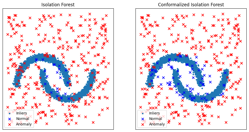
By calibrating the detection threshold, it is clear from the figure above that conformal anomaly detection reduces false alarms rate.